

Lab disclosure: This is a controlled portfolio case using synthetic customers and business scenarios. The analysis is based on 1,000 real OpenAI API requests and official usage and cost exports. No client data was used.
The business problem
As AI products scale, the provider invoice shows how much the company spent, but it rarely answers the questions needed for operational decision-making. For example, which workloads generate the most cost? Which customers consume the most AI resources? Is an expensive model being used for a workload where a smaller model may be sufficient? Are output limits affecting response completion? Can internal cost allocations be reconciled to the provider’s official records (the invoice)?
Without any level of specificity Finance sees a growing AI bill while Product and Engineering lack a shared view of the drivers behind it. This is where request-level cost tracking comes into the rescue.
This case demonstrates how an AI cost-control layer can connect the provider billing data with the detailed AI request records (also called telemetry) and convert them into practical cost-optimization decisions.
Scope of the analysis
The controlled case processed 1,000 requests through the OpenAI API using synthetic customers along with specific business scenarios. The requests were distributed across 10 customers, five representative business workloads and three model tiers.
The workloads were selected to reflect different ways a growing company might use AI in daily operations. The Support Chat workload, for example, handled customer questions and troubleshooting. Document Assistant answered questions using supplied document extracts. Ticket Classification assigned categories, priorities and routing teams to incoming requests. Contract Analyzer reviewed contract clauses for financial and commercial risks, while Background Summarization converted customer-success updates into concise internal summaries.
Together, these workloads allowed the analysis to examine how model selection, response length, latency and completion status influenced AI cost under different operational requirements.
The models were presented as Model A, Model B and Model C. Model A represented GPT-4.1 Nano, Model B represented GPT-4.1 Mini, and Model C represented GPT-4.1.
For every request, the analysis recorded the customer, the workload, the requested and resolved model, the input and the output tokens, the latency, the completion status and the estimated cost. These automatically recorded request details are referred to as telemetry.
How the workload and model mix was created
The 1,000 requests were created in two stages. First, 50 distinct business scenarios were prepared, with 10 scenarios for each of the 5 workloads. Every scenario was sent once to each of the 3 models. This produced 150 benchmark requests and ensured that all models were tested across all workloads.
The remaining 850 requests formed a simulated production mix. For each request, the model was selected using predefined probabilities based on the workload. This created an uneven but controlled distribution similar to what could occur when a company uses different models for different types of work.
The initial logic was to assign most routine and high-volume tasks to Model A, use Model B as the main option for tasks with moderate complexity, and use Model C less frequently, with a higher allocation to Contract Analyzer.
This distribution was an initial assumption made for the simulation. It was not based on measured output quality and should not be interpreted as the optimal model choice for each workload. Its purpose was to create a plausible starting pattern that could then be analysed and challenged through the model-routing scenario.

Table 1 above shows that Model C processed 104 requests. Out of them, 29 belonged to Contract Analyzer, while the remaining 75 belonged to Support Chat, Document Assistant, Ticket Classification and Background Summarization. These 75 requests form the balanced model-routing scenario presented later in the analysis.
Data model and methodology
The analysis combined two data layers.
The first layer was the operational request log (the details of each request or telemetry), which provided the business context missing from the provider exports. It showed which customer and workload generated each request, which model processed it, how many tokens were consumed, how long the response took and whether it was completed successfully.
The second layer consisted of the official OpenAI usage and cost exports. These files provided the control totals used to confirm that the request-level calculations matched the provider’s records.
A Power BI star schema connected the request log and official exports through shared model and date dimensions. The customer and workload dimensions were connected to the operational request data. In addition, this structure allowed the dashboard to use the official exports as a billing control while using the request records to analyse cost by customer, workload and model.
Reconciliation result
Before analysing the cost drivers, the operational records were reconciled to the official provider data. The results matched exactly:
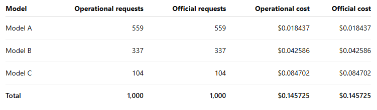
Request variance and cost variance were zero for every model.
This control is important because cost allocations by customer and workload are useful only when they reconcile to the official bill.
Executive overview
The executed case generated 1,000 requests, with 68,649 input tokens and 66,134 output tokens. Total token usage reached 134,783, while the total AI cost was $0.1457. The average cost per request was $0.000146, and the average response time was 1,371 milliseconds.
Of the 1,000 requests, 993 were completed successfully and seven were marked as incomplete as they reached a pre-configured output limit (explained later) . There were no hard API errors and no cached input tokens.
The absolute spend is low because this is a controlled benchmark. The important results are the differences in unit cost, the connection between cost and business activity, and the percentage-based optimization opportunities that could become material at production scale.

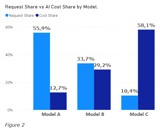
Finding 1: Model C generated 58.1% of cost from 10.4% of requests
Model C processed only 104 of the 1,000 requests but generated $0.084702of the $0.145725 total cost (or 58% of the total cost). Also displayed in Figure 2 below.
At the observed token volumes, an average Model C request cost approximately 6.4 times more than a Model B request and 24.7 times more than a Model A request.
This does not mean that Model C should be removed. A stronger and more expensive model may be justified when the task is complex or the cost of an incorrect answer is high. The result shows that Model C should be used selectively and connected to workloads where its additional capability creates measurable value.
Finding 2: The Contract Analyzer workload was the primary cost and latency driver
The Contract Analyzer workload generated approximately $0.0668, representing 46% of the total AI cost. Its average cost was $0.0006 per request, and its average response time was 2,013 milliseconds. Both figures were the highest among the five workloads. As shown in Figure 3 and Figure 4 below, Contract Analyzer ranked first for both average cost per request and average latency.
The workload included 115 requests: 13 were processed by Model A, 73 by Model B and 29 by Model C. Its higher cost reflected the greater use of Models B and C, together with the larger 450-token output limit used for contract analysis.
Because the model allocation was predefined for the simulation, the analysis measured cost, token usage, latency and completion but did not formally compare the output quality of Model B and Model C for this workload. The simulation therefore shows that Contract Analyzer was expensive under the tested model mix, but it does not establish that Model C is necessary to deliver acceptable results. A separate quality evaluation is required before a final routing decision can be made.


Finding 3: Output limits created an operational failure signal
Seven requests were marked as incomplete. All of them occurred within the Support Chat workload and reached the configured 160-token output limit.
The incomplete rate was 0.70% across the full benchmark and 2.12% within Support Chat. There were no hard API errors. The requests were processed and generated cost, but the models could not complete their responses within the configured output limit. Figure 4 shows how the 7 incomplete requests were distributed across the three models.
This problem would not be visible from the total AI invoice. It shows why cost information should be reviewed together with operational results.
Simply increasing the output limit for every workload would not be an efficient solution. A better approach would apply different limits based on the expected response length, monitor incomplete responses and use controlled retries only when additional output is necessary.
Finding 4: Cached tokens were zero
The simulation recorded no cached input tokens. Figure 4 below also confirms that cached input tokens remained at zero throughout the benchmark. However, the average request contained only 68.6 input tokens, so this dataset does not provide enough evidence to claim that prompt caching would create a meaningful saving.
Prompt caching is more relevant when production requests contain long and repeated prompt sections. It should not be presented as a guaranteed optimization without first reviewing the actual prompt structure and usage pattern.

Model-routing scenario
For the purposes of this analysis we identified model routing as the most important potential optimization. The scenario uses the recorded input and output token counts from the 1,000 requests. For selected requests originally processed by Model C, it recalculates what they would have cost at Model B prices.
This isolates the price effect of changing the model. It does not assume that Model B would use fewer tokens or produce the same quality. The result is therefore a financial scenario rather than a realized saving.
